Note
Go to the end to download the full example code
Design Matrix
This tutorial illustrates how to use the Design_Matrix class to flexibly create design matrices that can then be used with the Brain_Data class to perform univariate regression.
Design Matrices can be thought of as “enhanced” pandas dataframes; they can do everything a pandas dataframe is capable of, with some added features. Design Matrices follow a data organization format common in many machine learning applications such as the sci-kit learn API: 2d tables organized as observations by features. In the context of neuro-imaging this often translates to TRs by conditions of interest + nuisance covariates (1st level analysis), or participants by conditions/groups (2nd level analysis).
Design Matrix Basics
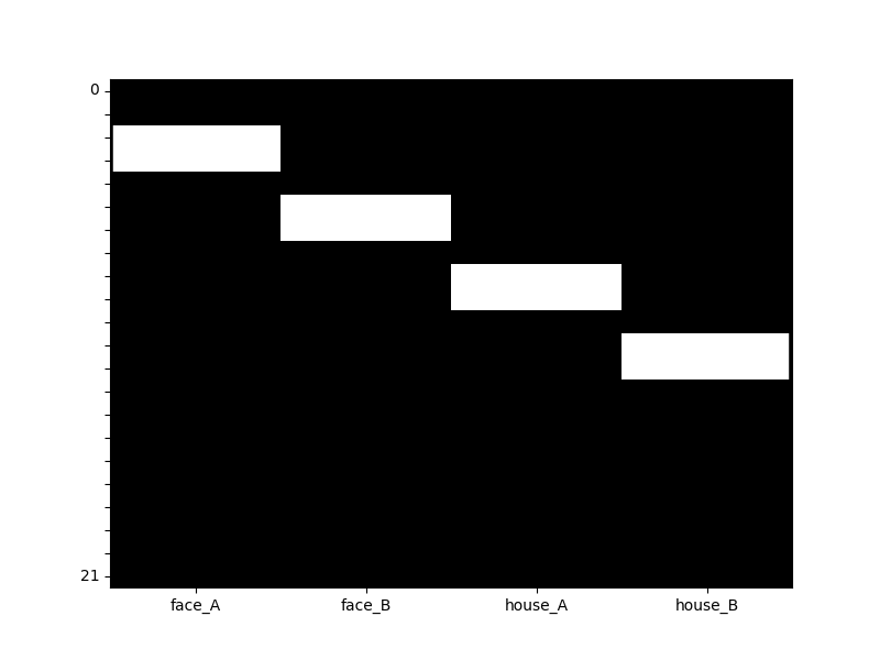
Lets just create a basic toy design matrix by hand corresponding to a single participant’s data from an experiment with 12 TRs, collected at a temporal resolution of 1.5s. For this example we’ll have 4 unique “stimulus conditions” that each occur for 2 TRs (3s) with 1 TR (1.5s) of rest between events.
from nltools.data import Design_Matrix
import numpy as np

TR = 1.5 # Design Matrices take a sampling_freq argument specified in hertz which can be converted as 1./TR

dm = Design_Matrix(np.array([
                            [0,0,0,0],
                            [0,0,0,0],
                            [1,0,0,0],
                            [1,0,0,0],
                            [0,0,0,0],
                            [0,1,0,0],
                            [0,1,0,0],
                            [0,0,0,0],
                            [0,0,1,0],
                            [0,0,1,0],
                            [0,0,0,0],
                            [0,0,0,1],
                            [0,0,0,1],
                            [0,0,0,0],
                            [0,0,0,0],
                            [0,0,0,0],
                            [0,0,0,0],
                            [0,0,0,0],
                            [0,0,0,0],
                            [0,0,0,0],
                            [0,0,0,0],
                            [0,0,0,0]
                            ]),
                            sampling_freq = 1./TR,
                            columns=['face_A','face_B','house_A','house_B']
                            )
Notice how this look exactly like a pandas dataframe. That’s because design matrices are subclasses of dataframes with some extra attributes and methods.
print(dm)
    face_A  face_B  house_A  house_B
0        0       0        0        0
1        0       0        0        0
2        1       0        0        0
3        1       0        0        0
4        0       0        0        0
5        0       1        0        0
6        0       1        0        0
7        0       0        0        0
8        0       0        1        0
9        0       0        1        0
10       0       0        0        0
11       0       0        0        1
12       0       0        0        1
13       0       0        0        0
14       0       0        0        0
15       0       0        0        0
16       0       0        0        0
17       0       0        0        0
18       0       0        0        0
19       0       0        0        0
20       0       0        0        0
21       0       0        0        0
Let’s take a look at some of that meta-data. We can see that no columns have been convolved as of yet and this design matrix has no polynomial terms (e.g. such as an intercept or linear trend).
print(dm.details())
nltools.data.design_matrix.Design_Matrix(sampling_freq=0.6666666666666666 (hz), shape=(22, 4), multi=False, convolved=[], polynomials=[])
We can also easily visualize the design matrix using an SPM/AFNI/FSL style heatmap
dm.heatmap()
Adding nuisiance covariates
Legendre Polynomials
A common operation is adding an intercept and polynomial trend terms (e.g. linear and quadtratic) as nuisance regressors. This is easy to do. Consistent with other software packages, these are orthogonal Legendre poylnomials on the scale -1 to 1.
# with include_lower = True (default), 2 here means: 0-intercept, 1-linear-trend, 2-quadtratic-trend
dm_with_nuissance = dm.add_poly(2,include_lower=True)
dm_with_nuissance.heatmap()
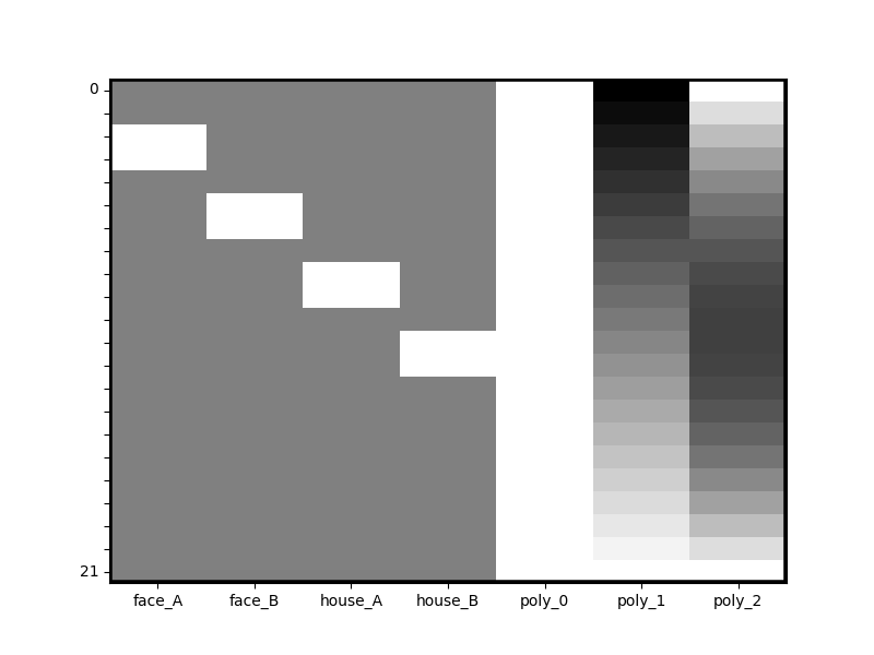
We can see that 3 new columns were added to the design matrix. We can also inspect the change to the meta-data. Notice that the Design Matrix is aware of the existence of three polynomial terms now.
print(dm_with_nuissance.details())
nltools.data.design_matrix.Design_Matrix(sampling_freq=0.6666666666666666 (hz), shape=(22, 7), multi=False, convolved=[], polynomials=['poly_0', 'poly_1', 'poly_2'])
Discrete Cosine Basis Functions
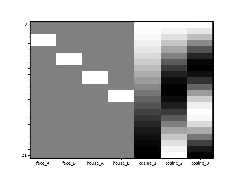
Polynomial variables are not the only type of nuisance covariates that can be generated for you. Design Matrix also supports the creation of discrete-cosine basis functions ala SPM. This will create a series of filters added as new columns based on a specified duration, defaulting to 180s. Let’s create DCT filters for 20s durations in our toy data.
# Short filter duration for our simple example
dm_with_cosine = dm.add_dct_basis(duration=20)
dm_with_cosine.heatmap()
Data operations
Performing convolution
Design Matrix makes it easy to perform convolution and will auto-ignore all columns that are consider polynomials. The default convolution kernel is the Glover (1999) HRF parameterized by the glover_hrf implementation in nipy (see nltools.externals.hrf for details). However, any arbitrary kernel can be passed as a 1d numpy array, or multiple kernels can be passed as a 2d numpy array for highly flexible convolution across many types of data (e.g. SCR).
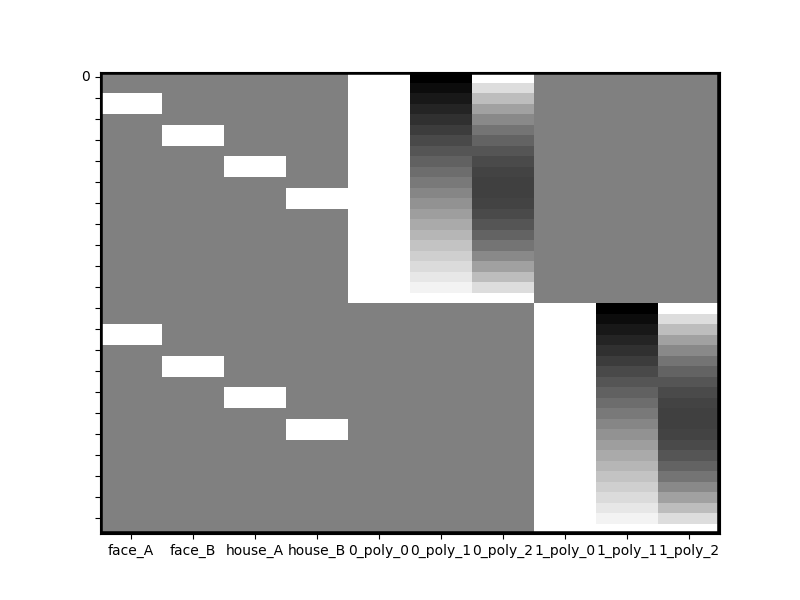
dm_with_nuissance_c = dm_with_nuissance.convolve()
print(dm_with_nuissance_c.details())
dm_with_nuissance_c.heatmap()
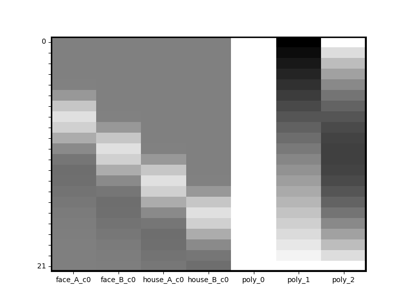
nltools.data.design_matrix.Design_Matrix(sampling_freq=0.6666666666666666 (hz), shape=(22, 7), multi=False, convolved=['face_A', 'face_B', 'house_A', 'house_B'], polynomials=['poly_0', 'poly_1', 'poly_2'])
Design Matrix can do many different data operations in addition to convolution such as upsampling and downsampling to different frequencies, zscoring, etc. Check out the API documentation for how to use these methods.
File Reading
Creating a Design Matrix from an onsets file
Nltools provides basic file-reading support for 2 or 3 column formatted onset files. Users can look at the onsets_to_dm function as a template to build more complex file readers if desired or to see additional features. Nltools includes an example onsets file where each event lasted exactly 1 TR and TR = 2s. Lets use that to create a design matrix with an intercept and linear trend
from nltools.utils import get_resource_path
from nltools.file_reader import onsets_to_dm
from nltools.data import Design_Matrix
import os

TR = 2.0
sampling_freq = 1./TR
onsetsFile = os.path.join(get_resource_path(),'onsets_example.txt')
dm = onsets_to_dm(onsetsFile, sampling_freq=sampling_freq, run_length=160, sort=True,add_poly=1)
dm.heatmap()

/home/runner/work/nltools/nltools/nltools/file_reader.py:79: UserWarning: Only 2 columns in file, assuming all stimuli are the same duration
  warnings.warn(
Creating a Design Matrix from a generic csv file
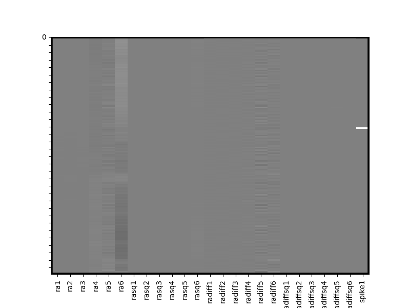
Alternatively you can read a generic csv file and transform it into a Design Matrix using pandas file reading capability. Here we’ll read in an example covariates file that contains the output of motion realignment estimated during a fMRI preprocessing pipeline.
import pandas as pd

covariatesFile = os.path.join(get_resource_path(),'covariates_example.csv')
cov = pd.read_csv(covariatesFile)
cov = Design_Matrix(cov, sampling_freq =sampling_freq)
cov.heatmap(vmin=-1,vmax=1) # alter plot to scale of covs; heatmap takes Seaborn heatmap arguments
Working with multiple Design Matrices
Vertically “stacking” Design Matrices
A common task is creating a separate design matrix for multiple runs of an experiment, (or multiple subjects) and vertically appending them to each other so that regression can be performed across all runs of an experiment. However, in order to account for run-differences its important (and common practice) to include separate run-wise polynomials (e.g. intercepts). Design Matrix’s append method is intelligent and flexible enough to keep columns separated during appending automatically.
# Lets use the design matrix with polynomials from above
# Stack "run 1" on top of "run 2"
runs_1_and_2 = dm_with_nuissance.append(dm_with_nuissance,axis=0)
runs_1_and_2.heatmap()
Separating columns during append operations
Notice that all polynomials have been kept separated for you automatically and have been renamed to reflect the fact that they come from different runs. But Design Matrix is even more flexible. Let’s say you want to estimate separate run-wise coefficients for all house stimuli too. Simply pass that into the unique_cols parameter of append.
runs_1_and_2 = dm_with_nuissance.append(dm_with_nuissance,unique_cols=['house*'],axis=0)
runs_1_and_2.heatmap()
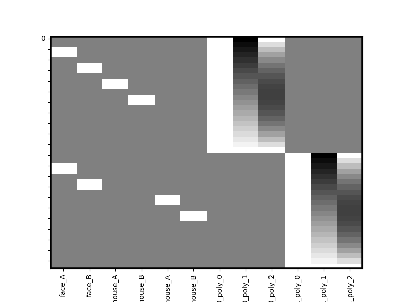
Now notice how all stimuli that begin with ‘house’ have been made into separate columns for each run. In general unique_cols can take a list of columns to keep separated or simple wild cards that either begin with a term e.g. “house*” or end with one “*house”.
Putting it all together
A realistic workflow
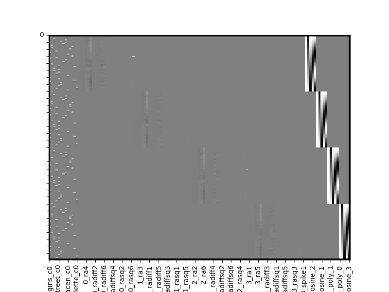
Let’s combine all the examples above to build a work flow for a realistic first-level analysis fMRI analysis. This will include loading onsets from multiple experimental runs, and concatenating them into a large multi-run design matrix where we estimate a single set of coefficients for our variables of interest, but make sure we account for run-wise differences nuisiance covarites (e.g. motion) and baseline, trends, etc. For simplicity we’ll just reuse the same onsets and covariates file multiple times.
num_runs = 4
TR = 2.0
sampling_freq = 1./TR
all_runs = Design_Matrix(sampling_freq = sampling_freq)
for i in range(num_runs):

    # 1) Load in onsets for this run
    onsetsFile = os.path.join(get_resource_path(),'onsets_example.txt')
    dm = onsets_to_dm(onsetsFile, sampling_freq=sampling_freq,run_length=160,sort=True)

    # 2) Convolve them with the hrf
    dm = dm.convolve()

    # 2) Load in covariates for this run
    covariatesFile = os.path.join(get_resource_path(),'covariates_example.csv')
    cov = pd.read_csv(covariatesFile)
    cov = Design_Matrix(cov, sampling_freq = sampling_freq)

    # 3) In the covariates, fill any NaNs with 0, add intercept and linear trends and dct basis functions
    cov = cov.fillna(0)

    # Retain a list of nuisance covariates (e.g. motion and spikes) which we'll also want to also keep separate for each run
    cov_columns = cov.columns
    cov = cov.add_poly(1).add_dct_basis()

    # 4) Join the onsets and covariates together
    full = dm.append(cov,axis=1)

    # 5) Append it to the master Design Matrix keeping things separated by run
    all_runs = all_runs.append(full,axis=0,unique_cols=cov.columns)

all_runs.heatmap(vmin=-1,vmax=1)
/home/runner/work/nltools/nltools/nltools/file_reader.py:79: UserWarning: Only 2 columns in file, assuming all stimuli are the same duration
  warnings.warn(
/home/runner/work/nltools/nltools/nltools/file_reader.py:79: UserWarning: Only 2 columns in file, assuming all stimuli are the same duration
  warnings.warn(
/home/runner/work/nltools/nltools/nltools/file_reader.py:79: UserWarning: Only 2 columns in file, assuming all stimuli are the same duration
  warnings.warn(
/home/runner/work/nltools/nltools/nltools/file_reader.py:79: UserWarning: Only 2 columns in file, assuming all stimuli are the same duration
  warnings.warn(
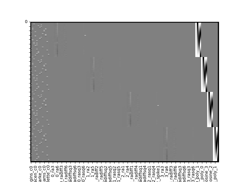
We can see the left most columns of our multi-run design matrix contain our conditions of interest (stacked across all runs), the middle columns includes separate run-wise nuisiance covariates (motion, spikes) and the right most columns contain run specific polynomials (intercept, trends, etc).
Data Diagnostics
Let’s actually check if our design is estimable. Design Matrix provides a few tools for cleaning up highly correlated columns (resulting in failure if trying to perform regression), replacing data, and computing collinearity. By default the clean method will drop any columns correlated at r >= .95
all_runs_cleaned = all_runs.clean(verbose=True)
all_runs_cleaned.heatmap(vmin=-1,vmax=1)
0_poly_1 and 0_cosine_1 correlated at 0.99 which is >= threshold of 0.95. Dropping 0_cosine_1
1_poly_1 and 1_cosine_1 correlated at 0.99 which is >= threshold of 0.95. Dropping 1_cosine_1
2_poly_1 and 2_cosine_1 correlated at 0.99 which is >= threshold of 0.95. Dropping 2_cosine_1
3_poly_1 and 3_cosine_1 correlated at 0.99 which is >= threshold of 0.95. Dropping 3_cosine_1
Whoops, looks like above some of our polynomials and dct basis functions are highly correlated, but the clean method detected that and dropped them for us. In practice you’ll often include polynomials or dct basis functions rather than both, but this was just an illustrative example.
Estimating a first-level model
You can now set this multi-run Design Matrix as the X attribute of a Brain_Data object containing EPI data for these four runs and estimate a regression in just a few lines of code.
# This code is commented because we don't actually have niftis loaded for the purposes of this tutorial
# See the other tutorials for more details on working with nifti files and Brain_Data objects

# Assuming you already loaded up Nifti images like this
# list_of_niftis = ['run_1.nii.gz','run_2.nii.gz','run_3.nii.gz','run_4.nii.gz']
# all_run_data = Brain_Data(list_of_niftis)

# Set our Design Matrix to the X attribute of Brain_Data object
# all_run_data.X = all_runs_cleaned

# Run the regression
# results = all_run_data.regress()

# This will produce N beta, t, and p images
# where N is the number of columns in the design matrix
Total running time of the script: (0 minutes 18.746 seconds)