Encoding Models

What it answers. How much of each voxel’s response can a stimulus feature space explain — on held-out data? An encoding model is the inverse of decoding: instead of predicting the stimulus from the brain, you predict the brain from features of the stimulus, and score each voxel by its cross-validated R².

For the theory, see the encoding-model material in naturalistic-data. This tutorial is about running one in nltools.

How it works. Compared with the GLM, an encoding model flips the question and the machinery:

GLM assumes a canonical HRF, uses a few categorical regressors, and asks which voxels respond (β / t / p).
Encoding uses many features (often hundreds), lets the data estimate the response shape, and asks how well features predict each voxel (cross-validated R²).

Two ideas make it work: a FIR (finite impulse response) feature bank — lagged copies of the stimulus, so ridge learns the per-voxel HRF instead of assuming one — and ridge regularization with per-voxel α, since hundreds of features would make ordinary least squares overfit. We compare an optimistic in-sample fit against an honest cross-validated one.

import numpy as np
from joblib import Memory

from nltools.data import BrainData
from nltools.utils import concatenate

# Memoize the (slow) multi-run load to disk (.cache/ is git-ignored).
memory = Memory(".cache/tutorials", verbose=0)

How to do it¶

We use the classic Miyawaki 2008 dataset — one subject viewing 10×10 binary contrast figures while we record from visual cortex. The stimulus is naturally 100-dimensional, so encoding is the right tool. The data ships in subject-native space (anisotropic voxels), so we pass mask= to skip MNI resampling and plot on the bundled anatomical with slice views (glass-brain/MNI views would misalign).

from nilearn.datasets import fetch_miyawaki2008

DATASET = fetch_miyawaki2008(verbose=0)

@memory.cache
def load_runs(n_runs: int):
    """Concatenate the first n_runs of BOLD and stack the matching stimulus."""
    runs = [BrainData(DATASET.func[i], mask=DATASET.mask) for i in range(n_runs)]
    bold = concatenate(runs)
    stim = np.vstack(
        [
            np.loadtxt(DATASET.label[i], delimiter=",", dtype=int)
            for i in range(n_runs)
        ]
    ).astype(float)
    stim[stim < 0] = 0.0  # rest frames → no-patch
    return bold, stim

bold, stim = load_runs(8)
print(f"bold: {bold.shape}  (TRs, voxels)   stim: {stim.shape}  (TRs, 100 patches)")

bold: (1040, 5438)  (TRs, voxels)   stim: (1040, 100)  (TRs, 100 patches)

Each on-frame is a 10×10 binary contrast figure — these 100 patches are our features:

import matplotlib.pyplot as plt

on_frames = (stim.sum(axis=1) > 0).nonzero()[0]
stim_fig, stim_axes = plt.subplots(1, 4, figsize=(9, 2.6))
for stim_ax, frame in zip(stim_axes, on_frames[:4]):
    stim_ax.imshow(stim[frame].reshape(10, 10), cmap="gray", vmin=0, vmax=1)
    stim_ax.set_title(f"TR {frame}")
    stim_ax.axis("off")
stim_fig.suptitle("Stimulus frames (10×10 binary contrast)", y=1.05)
stim_fig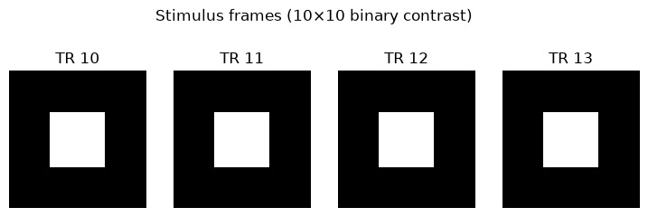

Build the feature matrix (FIR lag bank)¶

For each of the 100 patches we add copies at lags of 1, 2, and 3 TRs, giving 100 × 3 = 300 features. The weights ridge learns across those lags are an estimated impulse response per voxel — no canonical HRF assumed. Going from 100 to 300 features for ~1000 samples is exactly why we need ridge.

def lag_features(X, lags):
    """Stack lagged copies of X horizontally; pad early TRs with zeros."""
    n_tr, n_patch = X.shape
    out = np.zeros((n_tr, n_patch * len(lags)))
    for j, lag in enumerate(lags):
        out[lag:, j * n_patch : (j + 1) * n_patch] = X[: n_tr - lag]
    return out

X_fir = lag_features(stim, [1, 2, 3])
print(f"X_fir: {X_fir.shape}  (3 lags × 100 patches = 300 features)")

X_fir: (1040, 300)  (3 lags × 100 patches = 300 features)

Fit ridge: in-sample vs. cross-validated¶

Standard encoding preprocessing: demean each voxel (ridge here has no intercept) and skip the GLM’s percent-signal scaling (scale=False). A fixed-α fit with no CV gives ridge_scores — an in-sample R², which is optimistically biased.

bold.data = bold.data - bold.data.mean(axis=0, keepdims=True)  # voxelwise demean
bold.fit(model="ridge", X=X_fir, alpha=1.0, scale=False)
in_sample = bold.ridge_scores.data.ravel()
print(f"in-sample R²  — mean {in_sample.mean():.3f}  max {in_sample.max():.3f}")

in-sample R²  — mean 0.141  max 0.572

The honest version: alpha="auto" + cv=K sweeps an α grid and picks the best α per voxel (local_alpha=True, the default) — high-SNR visual voxels want little regularization, noisier voxels want more. cv_results_ then carries the cross-validated mean_score, per-fold scores, and selected best_alpha.

from sklearn.model_selection import KFold

ALPHAS = np.logspace(-1, 4, 20)
bold.fit(
    model="ridge",
    X=X_fir,
    alpha="auto",
    alphas=ALPHAS,
    cv=KFold(n_splits=5, shuffle=True, random_state=0),
    scale=False,
)
cv_r2 = bold.cv_results_["mean_score"]
print(f"CV R²        — mean {cv_r2.mean():.3f}  max {cv_r2.max():.3f}")
print(f"voxels with CV R² > 0.10: {(cv_r2 > 0.10).sum()} / {cv_r2.size}")

CV R²        — mean 0.102  max 0.552
voxels with CV R² > 0.10: 2213 / 5438

cv_map = bold.ridge_scores.copy()
cv_map.data = bold.cv_results_["mean_score"].reshape(1, -1)
cv_map.plot(
    method="slices",
    view="z",
    cut_coords=[[-12, -6, 0, 6, 12]],
    bg_img=DATASET.background,
    title="Ridge cross-validated R² (per-voxel α, FIR lags 1–3)",
    cmap="hot",
)

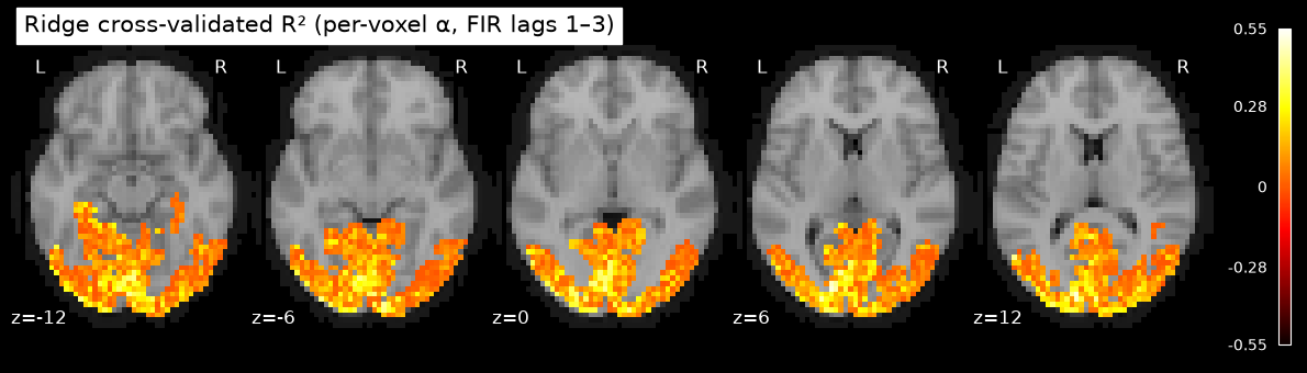
CV R² is smaller than in-sample (held-out is harder) and concentrates in the visual cortex that actually tracks the stimulus. Finally, the spread of selected α confirms why per-voxel regularization matters — voxels disagree:

best_alpha = np.asarray(bold.cv_results_["best_alpha"]).ravel()
alpha_fig, alpha_ax = plt.subplots(figsize=(7, 3))
alpha_ax.hist(np.log10(best_alpha), bins=len(ALPHAS), color="steelblue")
alpha_ax.set_xlabel(r"$\log_{10}(\alpha)$ selected per voxel")
alpha_ax.set_ylabel("voxel count")
alpha_ax.set_title("Per-voxel ridge α — voxels disagree on regularization")
alpha_fig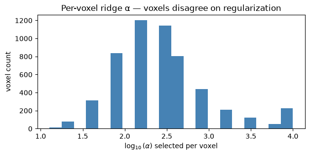

Recap¶

Stage	What it does	Key API
Load runs	Concatenate BOLD + stimulus across runs	`concatenate([...])`
Features	FIR lag bank (learn the HRF, don’t assume it)	`lag_features(stim, [1, 2, 3])`
In-sample fit	Fixed-α ridge → optimistic R²	`bold.fit(model="ridge", X=, alpha=1.0, scale=False)`
Honest fit	Per-voxel α via CV → out-of-sample R²	`bold.fit(model="ridge", X=, alpha="auto", alphas=, cv=)`
Inspect	CV R² map + selected α per voxel	`bold.cv_results_["mean_score"]`, `["best_alpha"]`

Next steps

GLM analysis — the inferential counterpart: which voxels respond.
Multivariate pattern analysis — decode the stimulus from brain patterns.
Inter-subject correlation — shared responses to naturalistic stimuli.