What it answers. Does the distributed pattern of activity across many voxels carry information about the conditions — beyond what any single voxel shows? Two complementary approaches:
Decoding — can a classifier predict the condition from the pattern? (cross-validated accuracy)
RSA — what is the geometry of the patterns relative to one another, and does it match a hypothesis? (a representational dissimilarity matrix compared to a model)
Both run at three spatial scales via spatial_scale= — 'whole_brain', 'roi', 'searchlight' — and either within a subject (here) or across subjects (loop + group test). For the theory, see dartbrains.
How it works. Both approaches operate on the same patterns; they differ in the question. Decoding fits a classifier across voxels and scores it on held-out data. RSA turns patterns into a distance matrix (the RDM) and correlates that geometry with a model RDM. The spatial_scale= switch is shared: whole-brain uses every voxel jointly, ROI runs the analysis per parcel, and searchlight sweeps a roving sphere.
We use the classic Haxby dataset — one subject viewing 8 object categories — for both.
import warnings

import numpy as np
import pandas as pd
from joblib import Memory

from nltools.data import Adjacency, BrainData
from nltools.templates import fetch_resource

memory = Memory(".cache/tutorials", verbose=0)
warnings.filterwarnings("ignore", message="Cannot detect name collisions")Decoding
Load Haxby (BrainData auto-resamples to MNI 3mm, so the bundled MNI atlas and searchlight line up), then restrict to face vs. house — the strongest, best-understood contrast. Boolean-indexing a BrainData slices its timeseries like a numpy array.
from nilearn.datasets import fetch_haxby

HAXBY = fetch_haxby(subjects=[2], verbose=0)

LABELS = pd.read_csv(HAXBY.session_target[0], sep=r"\s+")["labels"].to_numpy()

@memory.cache
def load_haxby_mni():
    """Load + MNI-resample the Haxby BOLD (slow; cached to disk)."""
    return BrainData(HAXBY.func[0])

brain = load_haxby_mni()
keep = np.isin(LABELS, ["face", "house"])
trials = brain[keep]
y = (LABELS[keep] == "face").astype(int)
print(
    f"trials: {trials.shape}  (n_trials, n_voxels)   classes (house, face): {np.bincount(y)}"
)
/home/runner/work/nltools/nltools/nltools/data/braindata/io.py:568: UserWarning:
Data resolution (3.667mm) doesn't exactly match template: default 3mm.
data_img = detect_and_update_mask(bd, data_img)
/home/runner/work/nltools/nltools/nltools/data/braindata/io.py:136: UserWarning: The provided image has no sform in its header. Please check the provided file. Results may not be as expected.
  return resample_to_img(
/home/runner/work/nltools/nltools/nltools/data/braindata/io.py:136: UserWarning: Casting data from int16 to float32
  return resample_to_img(
trials: (216, 71020) (n_trials, n_voxels) classes (house, face): [108 108]
Whole-brain
BrainData.predict() mirrors .fit(): one call, one frozen Predict result. cv scores generalization; weight_map is the classifier refit on all the data (the publishable map). For a linear SVM:
decode_wb = trials.predict(y=y, spatial_scale="whole_brain", model="svm", cv=5)
print(
    f"whole-brain accuracy: {decode_wb.mean_score:.3f} ± {decode_wb.std_score:.3f}  (chance 0.5)"
)
decode_wb.weight_map.plot(
    method="slices",
    title="SVM weights: + favors face, − favors house",
    cmap="RdBu_r",
    colorbar=True,
)
whole-brain accuracy: 0.986 ± 0.011 (chance 0.5)

Raw classifier weights are not a statistical map — a near-zero weight can still carry information other voxels already supply (see Haufe et al., 2014). For a cleaner “where”, decode per region.
ROI
spatial_scale="roi" with a parcellation trains one classifier per parcel and returns an accuracy_map — every voxel in parcel i filled with parcel i’s cross-validated accuracy. We use the bundled k50 atlas (matches our 3mm MNI space).
atlas_path = fetch_resource("masks/default/3mm-MNI152-2009fsl-k50.nii.gz")
decode_roi = trials.predict(
    y=y, spatial_scale="roi", roi_mask=atlas_path, model="svm", cv=5, n_jobs=4
)
print(
    f"per-parcel accuracy: {decode_roi.mean_score.shape[0]} parcels, best = {decode_roi.mean_score.max():.3f}"
)
decode_roi.accuracy_map.plot(
    method="slices",
    title="ROI decoding accuracy (chance 0.5)",
    cmap="RdBu_r",
    vmin=0.3,
    vmax=0.7,
    colorbar=True,
)
per-parcel accuracy: 50 parcels, best = 0.991
/home/runner/work/nltools/nltools/nltools/data/braindata/plotting.py:308: UserWarning: Non-finite values detected. These values will be replaced with zeros.
  display_slice = plot_stat_map(

Ventro-temporal cortex lights up — where face- and place-selective patches live. ROI accuracy answers “is this region informative on its own?”, a cleaner “where” than the joint whole-brain weights.
Searchlight
A roving sphere: one classifier per voxel-neighborhood, giving a per-voxel accuracy map. Same call, spatial_scale="searchlight". This fits thousands of classifiers, so it’s the slow one — we cache it.
@memory.cache
def searchlight_decode(radius_mm):
    return trials.predict(
        y=y,
        spatial_scale="searchlight",
        radius_mm=radius_mm,
        model="svm",
        cv=5,
        n_jobs=-1,
    )

decode_sl = searchlight_decode(8.0)
decode_sl.accuracy_map.plot(
    method="slices",
    title="Searchlight decoding accuracy (8 mm sphere)",
    cmap="hot",
    colorbar=True,
)
RSA
Decoding asks can we separate the conditions; RSA asks what is their geometry. Build one pattern per category (mean BOLD across that category’s TRs, shifted 2 TRs for the hemodynamic lag), then turn the patterns into a representational dissimilarity matrix (RDM).
conditions = [c for c in sorted(set(LABELS)) if c != "rest"]
shifted = np.roll(LABELS, 2)  # align BOLD to stimulus (~5s HRF lag)
patterns = np.vstack([brain.data[shifted == c].mean(axis=0) for c in conditions])
category_patterns = BrainData(patterns, mask=brain.mask)
print(
    f"category patterns: {category_patterns.shape}  ({len(conditions)} categories)"
)
category patterns: (8, 71020) (8 categories)
rdm = category_patterns.distance(metric="correlation")
rdm.labels = conditions
rdm.plot(cmap="RdBu_r")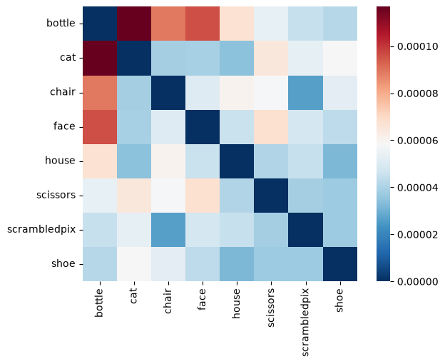
The RDM is the full geometry — every pairwise dissimilarity at once. To test a hypothesis, build a model RDM (here: animate face/cat vs. the rest) and correlate the two with a Mantel permutation test.
animate = np.array([c in ("face", "cat") for c in conditions])
model_rdm = Adjacency(
    (animate[:, None] != animate[None, :]).astype(float),
    matrix_type="distance",
    labels=conditions,
)
rsa_wb = rdm.similarity(
    model_rdm, metric="spearman", n_permute=1000, random_state=0
)
print(
    f"whole-brain RSA (animacy): rho = {rsa_wb['correlation']:.3f}  p = {rsa_wb['p']:.3f}"
)
whole-brain RSA (animacy): rho = 0.295 p = 0.249
Whole-brain, the animacy structure is weak — it’s diluted across regions that don’t represent categories. As with decoding, the signal is regional. spatial_scale="roi" computes one RDM per parcel, and project=True paints each parcel’s correlation-with-the-model back into brain space:
atlas_path_rsa = fetch_resource("masks/default/3mm-MNI152-2009fsl-k50.nii.gz")
roi_rdms = category_patterns.distance(
    metric="correlation", spatial_scale="roi", roi_mask=atlas_path_rsa
)
rsa_map = roi_rdms.similarity(
    model_rdm, metric="spearman", method=None, project=True
)
rsa_map.plot(
    method="slices",
    title="ROI RSA: where category geometry matches animacy",
    cmap="RdBu_r",
    colorbar=True,
)
Recap
Both approaches share the spatial_scale= axis, and both extend across subjects (loop per subject, then a group test on accuracies or projected RSA maps).
| Decoding | RSA | |
|---|---|---|
| Question | Can we predict the condition? | What’s the representational geometry? |
| Whole-brain | bd.predict(y=, spatial_scale="whole_brain") | bd.distance(metric="correlation") → .similarity(model) |
| ROI | bd.predict(y=, spatial_scale="roi", roi_mask=) | bd.distance(..., spatial_scale="roi", roi_mask=) → .similarity(model, project=True) |
| Searchlight | bd.predict(y=, spatial_scale="searchlight", radius_mm=) | bd.distance(..., spatial_scale="searchlight", radius_mm=) |
| Custom model | pass any sklearn estimator to model= | any metric= (spearman/pearson) |
Next steps
GLM analysis — the mass-univariate “where”, and how to build single-trial designs.
Encoding models — predict brain activity from stimulus features.
Inter-subject correlation — shared responses across people.