Adjacency Basics

The Adjacency class represents connectivity or similarity matrices. It stores data efficiently as the upper-triangle vector and reconstructs the full square matrix on demand. Common use cases:

Functional connectivity — correlations between ROI timeseries
Representational similarity — pattern-similarity matrices (RSA)
Behavioral similarity — subject-level similarity from traits or responses

It supports two matrix types: "similarity" (higher = more similar) and "distance" (higher = more dissimilar).

import numpy as np
import matplotlib.pyplot as plt

from nltools.data import Adjacency

Creating Adjacency objects¶

From a square matrix¶

n_nodes = 10

# A random symmetric matrix with a zero diagonal
_rng = np.random.default_rng(0)
random_matrix = _rng.standard_normal((n_nodes, n_nodes))
random_matrix = (random_matrix + random_matrix.T) / 2
np.fill_diagonal(random_matrix, 0)

adj = Adjacency(data=random_matrix, matrix_type="similarity")
print(adj)

nltools.data.adjacency.Adjacency(shape=(10, 10), Y=(0, 0), is_symmetric=True, matrix_type=similarity)

From brain data¶

BrainData.distance() computes pairwise distances between brain images and returns an Adjacency:

from nltools.datasets import fetch_pain

data = fetch_pain()

# A subset keeps the pairwise distance quick
subset = data[:20]
dist_matrix = subset.distance(metric="correlation")
print(f"Distance matrix: {dist_matrix.shape}")

Distance matrix: (20, 20)

Shape and storage¶

Adjacency distinguishes the logical shape (a square matrix) from the stored vector (its upper triangle):

print(f"Logical shape:   {adj.shape}")
print(f"Number of nodes: {adj.n_nodes}")
print(f"Vector length:   {adj.vector_shape}")
print(f"Expected n*(n-1)/2 = {n_nodes * (n_nodes - 1) // 2}")

Logical shape:   (10, 10)
Number of nodes: 10
Vector length:   (45,)
Expected n*(n-1)/2 = 45

Reconstruct the full matrix with squareform():

square = adj.squareform()
print(f"Square matrix: {square.shape}")
print(f"Symmetric:     {np.allclose(square, square.T)}")

Square matrix: (10, 10)
Symmetric:     True

Visualization¶

Heatmap¶

adj.plot()
_ = plt.gca().set_title("Random Similarity Matrix")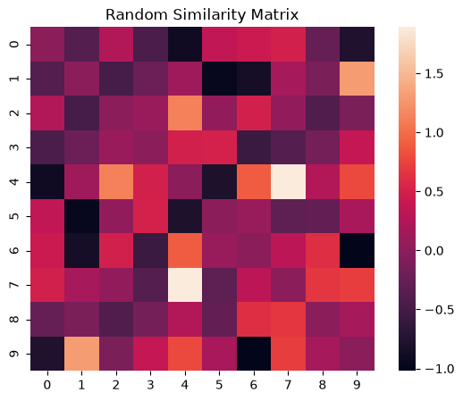

With labels¶

_roi_names = [f"ROI_{i}" for i in range(n_nodes)]
adj_labeled = Adjacency(
    data=random_matrix, matrix_type="similarity", labels=_roi_names
)
adj_labeled.plot()
_ = plt.gca().set_title("Labeled Matrix")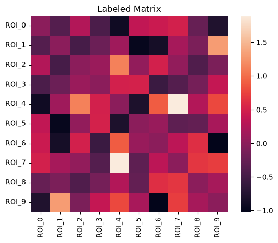

MDS plot¶

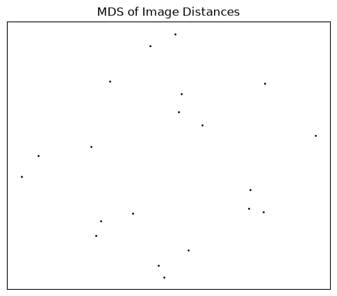
Multidimensional scaling lays out the structure of a distance matrix in 2D:

dist_matrix.plot_mds(n_components=2, figsize=(6, 5))
_ = plt.gca().set_title("MDS of Image Distances")

/home/runner/work/nltools/nltools/.venv/lib/python3.12/site-packages/sklearn/manifold/_mds.py:744: FutureWarning: The default value of `n_init` will change from 4 to 1 in 1.9. To suppress this warning, provide some value of `n_init`.
  warnings.warn(
/home/runner/work/nltools/nltools/.venv/lib/python3.12/site-packages/sklearn/manifold/_mds.py:754: FutureWarning: The default value of `init` will change from 'random' to 'classical_mds' in 1.10. To suppress this warning, provide some value of `init`.
  warnings.warn(
/home/runner/work/nltools/nltools/.venv/lib/python3.12/site-packages/sklearn/manifold/_mds.py:771: FutureWarning: The `dissimilarity` parameter is deprecated and will be removed in 1.10. Use `metric` instead.
  warnings.warn(
/home/runner/work/nltools/nltools/.venv/lib/python3.12/site-packages/sklearn/manifold/_mds.py:779: FutureWarning: Use metric_mds=True instead of metric=True. The support for metric={True/False} will be dropped in 1.10.
  warnings.warn(

Thresholding¶

Remove weak connections by absolute value or percentile, and optionally binarize:

# Absolute threshold: keep edges > 0.3
thresh = adj.threshold(lower=0.3)
print(f"Edges above 0.3: {(thresh.data > 0).sum()} / {len(thresh.data)}")

# Percentile threshold: keep the top 10%
thresh_pct = adj.threshold(lower="90%")
print(f"Top 10% edges:   {(thresh_pct.data > 0).sum()}")

# Binarize
binary = adj.threshold(lower=0.3, binarize=True)
print(f"Binary values:   {np.unique(binary.data)}")

Edges above 0.3: 10 / 45
Top 10% edges:   21
Binary values:   [0. 1.]

_fig, _axes = plt.subplots(1, 3, figsize=(15, 4))
adj.plot(axes=_axes[0])
_axes[0].set_title("Original")
thresh.plot(axes=_axes[1])
_axes[1].set_title("Thresholded (> 0.3)")
binary.plot(axes=_axes[2])
_axes[2].set_title("Binarized")
_fig.tight_layout()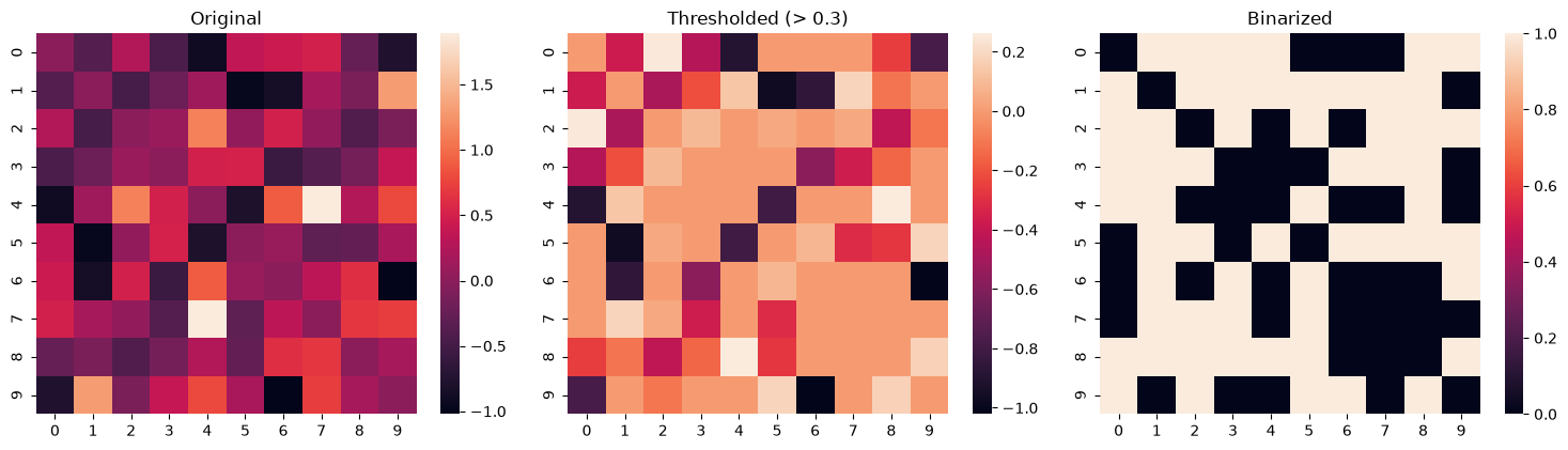

Statistics¶

Summary statistics¶

print(f"Mean:   {adj.mean():.4f}")
print(f"Std:    {adj.std():.4f}")
print(f"Median: {adj.median():.4f}")

Mean:   0.0783
Std:    0.6178
Median: 0.0961

Comparing two matrices¶

similarity() tests whether two matrices are related, with permutation-based inference:

# Two related matrices
_rng = np.random.default_rng(42)
_m1 = _rng.standard_normal((15, 15))
_m1 = (_m1 + _m1.T) / 2
np.fill_diagonal(_m1, 0)

_m2 = _m1 + _rng.standard_normal((15, 15)) * 0.5
_m2 = (_m2 + _m2.T) / 2
np.fill_diagonal(_m2, 0)

adj1 = Adjacency(_m1, matrix_type="similarity")
adj2 = Adjacency(_m2, matrix_type="similarity")

_result = adj1.similarity(adj2, metric="spearman", n_permute=5000)
print(f"Spearman r = {_result['correlation']:.3f}, p = {_result['p']:.4f}")

Spearman r = 0.848, p = 0.0002

Fisher’s r-to-z transform¶

When averaging or comparing correlation matrices, apply the Fisher transform first:

_rng = np.random.default_rng(7)
_corr_data = np.corrcoef(_rng.standard_normal((8, 50)))
np.fill_diagonal(_corr_data, 0)
corr_adj = Adjacency(_corr_data, matrix_type="similarity")

_z_adj = corr_adj.r_to_z()
print(f"Original range: [{corr_adj.data.min():.3f}, {corr_adj.data.max():.3f}]")
print(f"Z-scored range: [{_z_adj.data.min():.3f}, {_z_adj.data.max():.3f}]")

_r_adj = _z_adj.z_to_r()
print(f"Round-trip check: {np.allclose(corr_adj.data, _r_adj.data, atol=1e-10)}")

Original range: [-0.209, 0.272]
Z-scored range: [-0.212, 0.279]
Round-trip check: True

Arithmetic¶

Adjacency supports element-wise arithmetic:

_diff = adj1 - adj2
_scaled = adj1 * 2
print(f"Difference mean: {_diff.mean():.4f}")
print(f"Scaled mean:     {_scaled.mean():.4f}")

Difference mean: 0.0029
Scaled mean:     -0.0669

Application: functional connectivity¶

# Five ROI timeseries with a bit of correlation structure
_rng = np.random.default_rng(0)
_roi_ts = _rng.standard_normal((100, 5))
_roi_ts[:, 1] = (
    _roi_ts[:, 0] + _rng.standard_normal(100) * 0.3
)  # ROI 0-1 correlated
_roi_ts[:, 4] = (
    _roi_ts[:, 3] + _rng.standard_normal(100) * 0.3
)  # ROI 3-4 correlated

_fc_matrix = np.corrcoef(_roi_ts.T)
np.fill_diagonal(_fc_matrix, 0)

_roi_labels = ["DLPFC_L", "DLPFC_R", "ACC", "Insula_L", "Insula_R"]
fc = Adjacency(_fc_matrix, matrix_type="similarity", labels=_roi_labels)
fc.plot()
_ = plt.gca().set_title("ROI-to-ROI Functional Connectivity")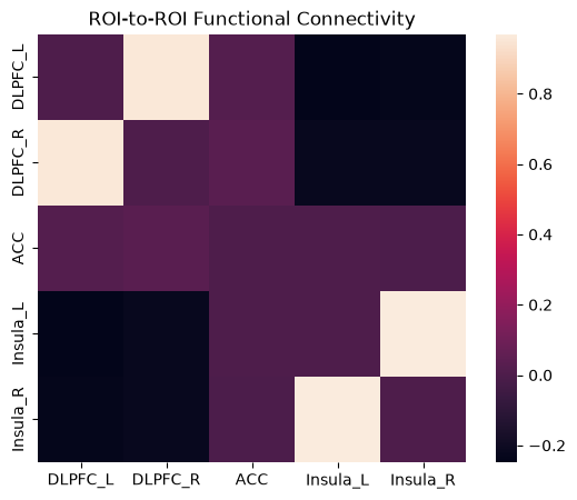

Application: representational similarity analysis¶

Simulate neural patterns with category structure — faces similar to faces, objects similar to objects — and build a representational dissimilarity matrix:

_rng = np.random.default_rng(1)
_patterns = _rng.standard_normal((6, 1000))
_patterns[1] = _patterns[0] + _rng.standard_normal(1000) * 0.2
_patterns[2] = _patterns[0] + _rng.standard_normal(1000) * 0.2
_patterns[4] = _patterns[3] + _rng.standard_normal(1000) * 0.2
_patterns[5] = _patterns[3] + _rng.standard_normal(1000) * 0.2

_rdm = 1 - np.corrcoef(_patterns)
np.fill_diagonal(_rdm, 0)

_labels = ["Face1", "Face2", "Face3", "Object1", "Object2", "Object3"]
rsa = Adjacency(_rdm, matrix_type="distance", labels=_labels)
rsa.plot()
_ = plt.gca().set_title("Representational Dissimilarity Matrix")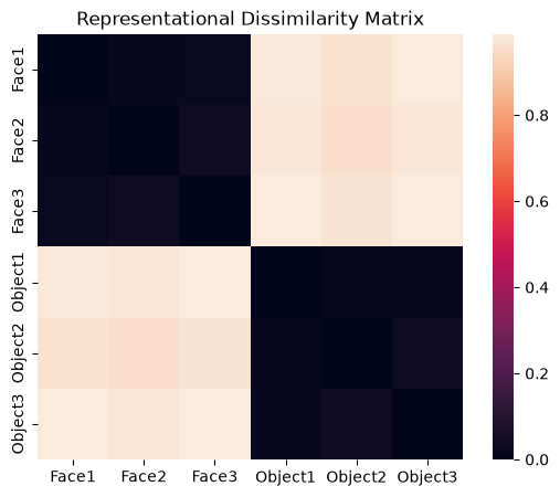

Notice the block-diagonal structure: faces are similar to faces (low dissimilarity), objects to objects.

Stacking multiple matrices¶

Use append() to stack matrices (e.g. one per subject) for group-level analysis:

# Simulate an FC matrix per subject
_rng = np.random.default_rng(3)
_matrices = []
for _ in range(5):
    _ts = _rng.standard_normal((100, 5))
    _ts[:, 1] = _ts[:, 0] + _rng.standard_normal(100) * 0.3
    _m = np.corrcoef(_ts.T)
    np.fill_diagonal(_m, 0)
    _matrices.append(Adjacency(_m, matrix_type="similarity"))

stacked = _matrices[0]
for _mat in _matrices[1:]:
    stacked = stacked.append(_mat)

print(f"Stacked: {len(stacked)} matrices, {stacked.n_nodes} nodes each")

_group_mean = stacked.mean()
print(f"Group mean shape: {_group_mean.shape}")

# One-sample t-test across subjects
_ttest = stacked.ttest()
print(f"T-test: {(_ttest['p'].data < 0.05).sum()} significant edges (p < 0.05)")

Stacked: 5 matrices, 5 nodes each
Group mean shape: (5, 5)
T-test: 1 significant edges (p < 0.05)

File I/O¶

import os
import tempfile

with tempfile.TemporaryDirectory() as _tmpdir:
    _path = os.path.join(_tmpdir, "adjacency.csv")
    adj.write(_path, method="square")
    print(f"Saved: {adj.shape}")

    _loaded = Adjacency(_path, matrix_type="similarity")
    print(f"Loaded: {_loaded.shape}")
    print(f"Round-trip check: {np.allclose(adj.data, _loaded.data)}")

Saved: (10, 10)
Loaded: (10, 10)
Round-trip check: True

Summary¶

In this tutorial you learned to:

Create Adjacency from square matrices, vectors, or BrainData.distance()
Store as an upper-triangle vector with squareform() reconstruction
Visualize with plot() heatmaps and plot_mds() for structure
Threshold by absolute value, percentile, and binarization
Test with mean(), ttest(), and similarity() permutation tests
Transform with r_to_z() / z_to_r() (Fisher transforms)
Stack with append() for group-level analysis

For a complete representational-similarity workflow, see the Multivariate Pattern Analysis tutorial, which builds an RDM from real brain patterns and compares it to a model.