The BrainData class is the core data structure in nltools for working with
neuroimaging data. It stores data as 2D arrays (images x voxels) for efficient
computation, automatically handles resampling to standard MNI space (default),
and supports standard Python operations like indexing, arithmetic, and iteration.
from nltools import BrainData

# Empty brain
BrainData()
nltools.data.braindata.BrainData(data=(0,), resolution=2.0mm, space=mni, mask=2mm-MNI152-2009fsl-mask.nii.gz)Loading data
You pass a file path, a nilearn/nibabel image, a file URL, or lists of any of
those to BrainData() — it loads and resamples to MNI space if needed, e.g.
BrainData('myfile.nii.gz').
To keep things simple we use one of the included datasets. fetch_pain()
downloads a pain-perception study (Chang et al., 2015): 28 subjects x 3
conditions = 84 images.
from nltools.datasets import fetch_pain

brains = fetch_pain()
The BrainData repr shows the shape (images x voxels) and whether metadata polars DataFrames (X, Y) are attached.
brainsnltools.data.braindata.BrainData(data=(84, 238955), resolution=2.0mm, space=mni, mask=2mm-MNI152-2009fsl-mask.nii.gz)Access the underlying data as a numpy array with the .data attribute:
brains.data.shape # (images, voxels)(84, 238955)BrainData also stores metadata as polars DataFrames on .X and .Y:
X: design matrix / covariates for modeling
Y: outcome variables or labels
# The pain dataset ships metadata in X
brains.X.head()Saving data
BrainData saves as NIfTI (.nii.gz) or HDF5 (.h5). HDF5 preserves metadata
(X, Y) and masks and produces smaller files:
brains.write("data.nii.gz")   # NIfTI
brains.write("data.h5")       # HDF5, with X/Y/mask/etc.
Indexing and slicing
BrainData supports standard Python-style indexing, and all indexing preserves
the X/Y metadata.
# Single image
brains[0]
nltools.data.braindata.BrainData(data=(238955,), resolution=2.0mm, space=mni, mask=2mm-MNI152-2009fsl-mask.nii.gz)# Slicing
first_five = brains[:5]
print(f"Sliced: {first_five.shape}")Sliced: (5, 238955)
# List indexing
selected = brains[[0, 10, 20, 30]]
print(f"Selected: {selected.shape}")
Selected: (4, 238955)
Boolean indexing filters images by computed properties:
# Filter images whose global mean exceeds twice their own global mean
# (illustrative boolean-mask indexing)
_global_mean = brains.mean(axis=1)
_keep = _global_mean > _global_mean.mean()
high_intensity = brains[_keep]
print(f"Images kept: {len(high_intensity)}")
Images kept: 35
Use .append() to concatenate BrainData objects:
# Append one image to another
brains[0].append(brains[1]).shape
(2, 238955)Arithmetic operations
BrainData supports element-wise arithmetic with scalars and other BrainData
objects.
# Addition (scalar, broadcast over every voxel)
brains + 100
nltools.data.braindata.BrainData(data=(84, 238955), resolution=2.0mm, space=mni, mask=2mm-MNI152-2009fsl-mask.nii.gz)# Subtraction of two images → single brain map
brains[1] - brains[0]nltools.data.braindata.BrainData(data=(238955,), resolution=2.0mm, space=mni, mask=2mm-MNI152-2009fsl-mask.nii.gz)# Adding two BrainData objects element-wise
brains + brainsnltools.data.braindata.BrainData(data=(84, 238955), resolution=2.0mm, space=mni, mask=2mm-MNI152-2009fsl-mask.nii.gz)Statistical operations
BrainData exposes many statistical methods that reduce across images
(axis=0) or across voxels (axis=1).
# Mean across all images → single brain map
brains.mean()
nltools.data.braindata.BrainData(data=(238955,), resolution=2.0mm, space=mni, mask=2mm-MNI152-2009fsl-mask.nii.gz)# Standard deviation across images → single brain map
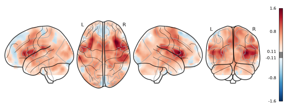
brains.std()nltools.data.braindata.BrainData(data=(238955,), resolution=2.0mm, space=mni, mask=2mm-MNI152-2009fsl-mask.nii.gz)# Temporal signal-to-noise ratio, then plot it
tsnr = brains.mean() / brains.std()
tsnr.plot()/home/runner/work/nltools/nltools/nltools/data/braindata/plotting.py:283: UserWarning: Non-finite values detected. These values will be replaced with zeros.
display_glass = plot_glass_brain(
# Standardization / z-scoring across images
z_scored = brains.standardize(method="zscore")
print(f"Z-scored mean: {z_scored.mean().data.mean():.6f}")
print(f"Z-scored std:  {z_scored.std().data.mean():.4f}")
Z-scored mean: 0.000000
Z-scored std: 0.9786
/home/runner/work/nltools/nltools/.venv/lib/python3.12/site-packages/sklearn/preprocessing/_data.py:273: UserWarning: Numerical issues were encountered when centering the data and might not be solved. Dataset may contain too large values. You may need to prescale your features.
  warnings.warn(
/home/runner/work/nltools/nltools/.venv/lib/python3.12/site-packages/sklearn/preprocessing/_data.py:292: UserWarning: Numerical issues were encountered when scaling the data and might not be solved. The standard deviation of the data is probably very close to 0.
  warnings.warn(
# Gaussian spatial smoothing at a given FWHM (mm)
_smoothed = brains[0].smooth(fwhm=6)
print(f"Original range: [{brains[0].data.min():.2f}, {brains[0].data.max():.2f}]")
print(f"Smoothed range: [{_smoothed.data.min():.2f}, {_smoothed.data.max():.2f}]")
Original range: [-2.86, 1.02]
Smoothed range: [-2.26, 0.38]
Threshold by absolute value or percentile, optionally binarizing for a mask:
# Keep only voxels in the top 5%
brains.mean().threshold(upper="95%").plot()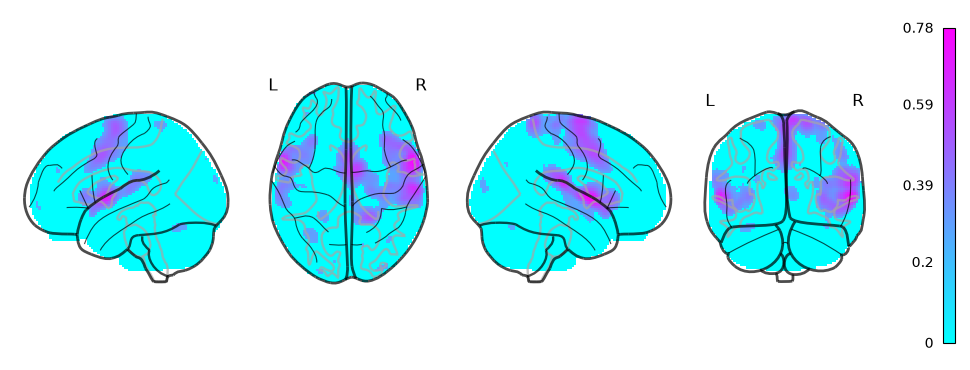
# Binarize for use as a mask
_binary_mask = brains.mean().threshold(upper="95%", binarize=True)
print(f"Mask voxels: {_binary_mask.data.sum():.0f}")
Mask voxels: 11693
Masking
Use apply_mask to restrict data to a region of interest.
# Mean map, with color bounds captured so later plots stay comparable
mean_brain = brains.mean()
vmin, vmax = mean_brain.data.min(), mean_brain.data.max()
mean_brain.plot(vmin=vmin, vmax=vmax)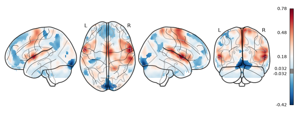
# An ROI mask from the top 10% of mean activation
roi_mask = mean_brain.threshold(upper="90%", binarize=True)
roi_mask.plot(vmin=0, vmax=1, cmap="gray_r")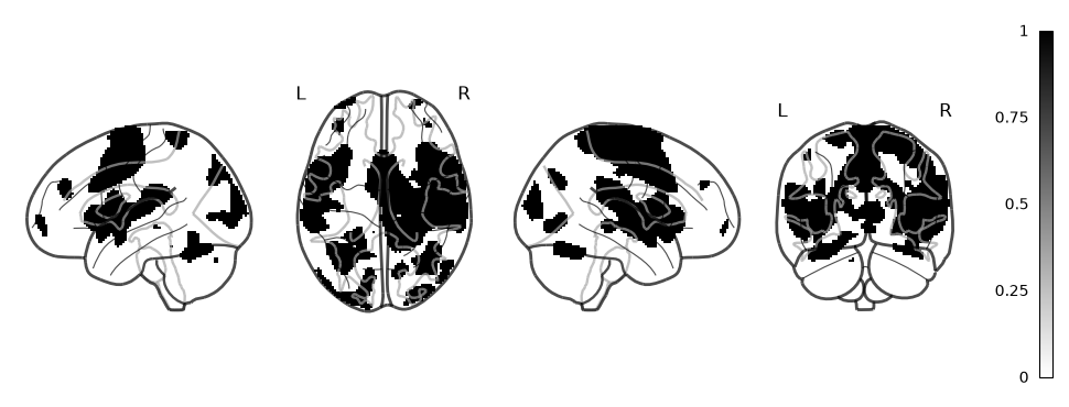
# Apply it — voxels outside the mask render transparent
masked_data = mean_brain.apply_mask(roi_mask)
masked_data.plot(vmin=vmin, vmax=vmax, cmap="RdBu_r")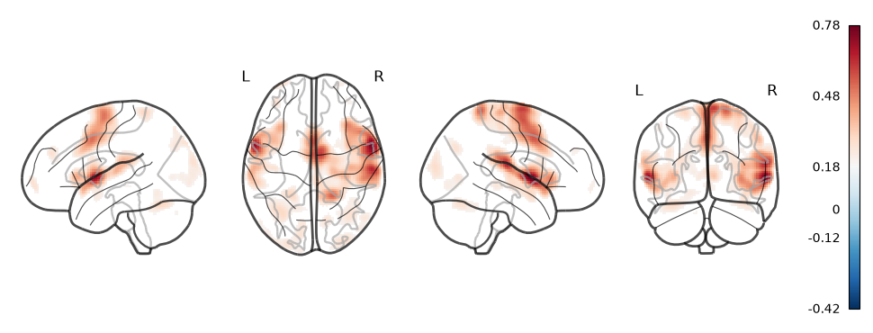
Visualization
BrainData.plot() supports several visualization types via the method
argument. Most wrap nilearn.plotting,
so you can always drop down to BrainData.to_nifti() and call nilearn directly.
Glass brain (default)
masked_data.plot(title="Mean Activation")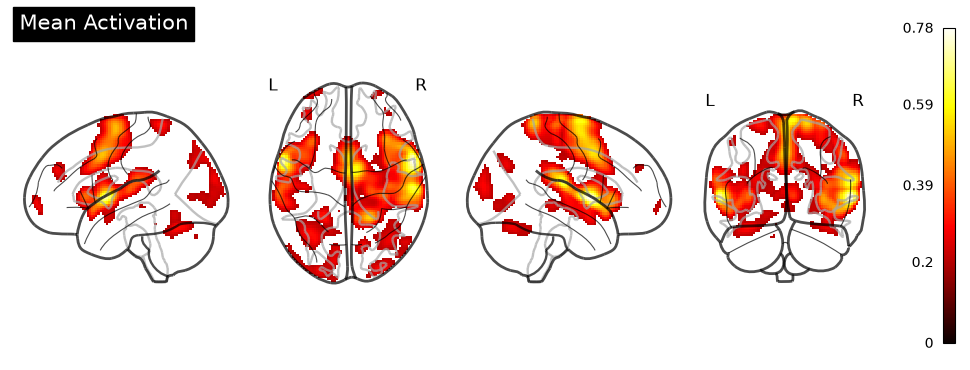
Slices
# Default: all views
masked_data.plot(method="slices")
# Only the Z view
masked_data.plot(method="slices", view="z")
Surface & flat-map
masked_data.plot_surf(zoom=1.3)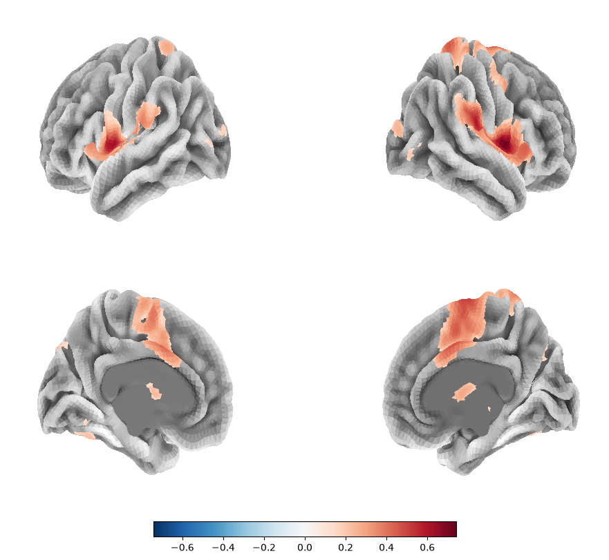
masked_data.plot_flatmap()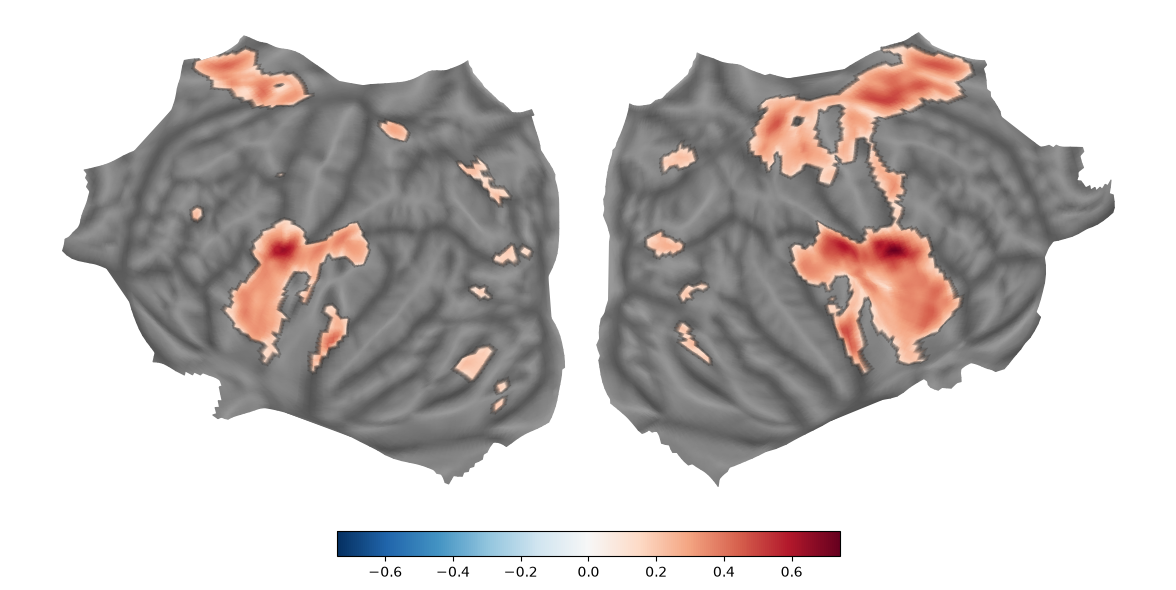
Timeseries & voxel distribution
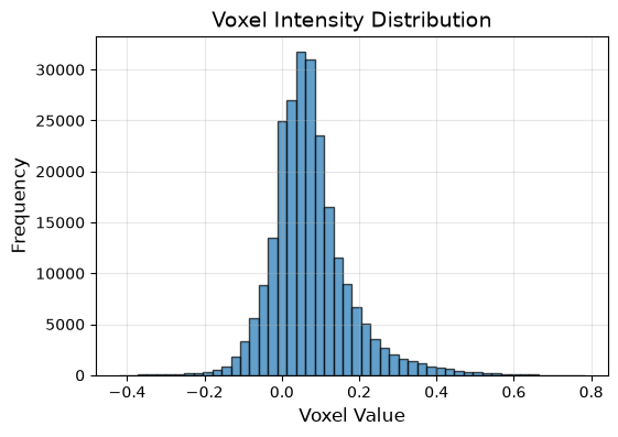
For multi-image BrainData, plot the mean signal over images; histogram shows
the voxel-intensity distribution.
brains.plot(method="timeseries", figsize=(6, 4))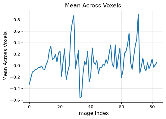
mean_brain.plot(
    method="histogram", title="Voxel Intensity Distribution", figsize=(6, 4)
)
Interactive viewer
BrainData.iplot() returns an interactive niivue viewer —
a WebGL anywidget that drives @niivue/niivue directly: a threshold slider
stacked above the viewer, with the stat-map colorbar shown. Drag the slider (or
right-drag on the image) to window the map live; scroll through slices, scrub 4D
frames, render in 3D, and overlay nltools atlases with hover-to-label. It speaks
anywidget’s standard model API, so it renders in any live kernel (marimo, Jupyter).
Pass controls=False to hide the slider (right-drag windowing still works), and
colorbar=False to hide the colorbar. No ipywidgets dependency needed.
# Interactive niivue viewer with a threshold slider (an anywidget driving
# @niivue/niivue directly, so it renders in any live kernel).
masked_data.iplot()