BrainCollection Basics

A BrainCollection is a parallel, memory-efficient iterator of BrainData — one BrainData per subject (or run). It saves you from writing for-loops over subjects: its API mirrors BrainData, but every per-subject operation (smooth, standardize, fit, ...) runs across all subjects in parallel, and group operations (mean, ttest, ...) reduce over subjects to a single BrainData map.

By default it is lazy and path-backed: subjects are loaded on demand and the results of parallel ops are streamed to a visible disk cache, so peak memory stays at roughly n_workers × 1 subject no matter how many subjects you have.

From a stack of images to a collection¶

To keep things self-contained we reuse the pain dataset from the BrainData tutorial: fetch_pain() returns a single BrainData of 84 images — 28 subjects × 3 stimulus-intensity conditions (low / medium / high) — with a metadata table in .X.

import polars as pl

from nltools.datasets import fetch_pain

stacked = fetch_pain()
stacked.X.select(["SubjectID", "PainIntensity", "Age", "Sex"]).head()

That stacked BrainData mixes all 28 subjects together. To analyze per subject we split it into one BrainData per subject (each holding that subject’s 3 condition maps) and wrap the list in a BrainCollection.

This explicit constructor takes a list[BrainData | path], a shared mask, and a per-subject metadata table. For real datasets on disk you’d usually skip the manual grouping and use a classmethod constructor instead:

• BrainCollection.from_bids(root, mask=...) — auto-pairs BOLD with events.tsv (→ DesignMatrix) and confounds.tsv from a BIDS derivatives tree.

• BrainCollection.from_glob("sub-*/beta.nii.gz", mask=...) — one item per matched file, with an optional design_pattern.

• BrainCollection.from_paths([...], mask=...) — explicit matched lists.

• BrainCollection.read(dir, mask=...) — inverse of bc.write(dir).

from nltools.data import BrainCollection

# One BrainData per subject (each = that subject's low/medium/high maps)
subject_ids = sorted(stacked.X["SubjectID"].unique().to_list())
per_subject = [
    stacked[[i for i, s in enumerate(stacked.X["SubjectID"]) if s == sid]]
    for sid in subject_ids
]

# One metadata row per subject (simple-typed columns only)
subject_meta = pl.DataFrame(
    [
        {
            "subject": f"sub-{sid:02d}",
            **stacked.X.filter(pl.col("SubjectID") == sid).row(0, named=True),
        }
        for sid in subject_ids
    ]
).select(["subject", "Age", "Sex"])

bc = BrainCollection(
    per_subject,
    mask=stacked.mask,
    metadata=subject_meta,
    cache_dir=None,  # ephemeral tempdir, auto-cleaned at exit
)
bc

The repr shows n_subjects and how many are currently loaded in memory (loaded=28/28 here, since we built it from in-memory BrainData; a collection built from paths starts cold at loaded=0/28).

Properties¶

BrainCollection exposes lightweight properties that don’t materialize the data.

# (n_subjects, images-per-subject, n_voxels). The middle dim is None when
# subjects have differing image counts.
bc.shape

print(f"n_subjects: {bc.n_subjects}")
print(f"n_voxels:   {bc.n_voxels}")
print(f"loaded:     {sum(bc.is_loaded)}/{bc.n_subjects}")
print(f"memory:     {bc.memory_estimate()}")
# memory_estimate() reports the full in-RAM footprint if every subject were loaded

n_subjects: 28
n_voxels:   238955
loaded:     28/28
memory:     BrainCollection(n_subjects=28, per_item=3×238955, estimated_total≈76.6 MB)

# Per-subject metadata as a polars DataFrame
bc.metadata.head()

Indexing and iteration¶

Indexing follows an intuitive rule: an integer or subject label returns a single BrainData; a slice, list, boolean mask, or polars expression returns a smaller BrainCollection (sharing the same cache root).

# Integer → the BrainData for that subject (3 condition maps)
bc[0]

# Subject label → BrainData, looked up via metadata['subject']
bc["sub-05"].shape

# Slice → a sub-collection
bc[:5]

# polars expression on metadata → filtered sub-collection
bc[pl.col("Sex") == "Female"]

# Iterate to get each subject's BrainData
per_subject_means = [bd.mean().data.mean() for bd in bc]
print(
    f"grand mean of {len(per_subject_means)} subject means: "
    f"{sum(per_subject_means) / len(per_subject_means):.3f}"
)

grand mean of 28 subject means: 0.073

Per-subject operations (parallel)¶

Every per-subject method mirrors the same method on BrainData, but runs across all subjects in parallel and returns a new BrainCollection. They all accept n_jobs, progress_bar, and cache.

Here we smooth every subject at 6 mm FWHM (the default n_jobs=-1 uses every core).

smoothed = bc.smooth(fwhm=6)
smoothed

map applies an arbitrary BrainData → BrainData function per subject, and apply calls a named BrainData method on every subject — the escape hatches when there’s no dedicated wrapper. Here we reduce each subject to just their high-pain map (the 3rd image), giving a single-map-per-subject collection.

high_pain = bc.map(lambda bd: bd[2])  # 3rd condition = "high"
high_pain.shape  # (28, n_voxels) — one map per subject

The memory model: path-backed by default¶

The collection built above lives in memory because we constructed it from in-memory BrainData. Constructors like from_bids instead return a lazy collection whose subjects are on disk, and parallel ops write their results through to a visible cache (./.nltools_cache/{run_id}/) rather than accumulating everything in RAM.

The cache= knob on every parallel op controls this:

bc.load() / bc.unload() move subjects between disk and RAM; bc.steps() lists the cache sub-directories produced so far; bc.cleanup() removes the whole cache root for this collection and its derived clones. Let’s force one op to disk and inspect the trail.

cached = bc.smooth(fwhm=6, cache=True)
print(f"result loaded in RAM? {any(cached.is_loaded)}")
print("cache steps:")
for step in cached.steps():
    print(f"  {step.name}")

result loaded in RAM? False
cache steps:
  20260902T004002_000000000_8601a858_smooth_fwhm-6

# A path-backed collection materializes on demand; load() pulls it into RAM
cached.load()
print(f"after load(): {sum(cached.is_loaded)}/{cached.n_subjects} in RAM")

after load(): 28/28 in RAM

Group reductions (collection → BrainData)¶

Reductions collapse the subject axis and return a single in-memory BrainData (or a dict of them). They stream from disk when the source is path-backed, so they stay memory-light.

mean() over our full collection averages each condition across subjects, giving a (3, n_voxels) map — one mean image per condition. We plot the mean high-pain map.

group_mean = bc.mean()  # (3, n_voxels): mean low / medium / high across subjects
group_mean[2].plot(title="Mean high-pain activation (n=28)")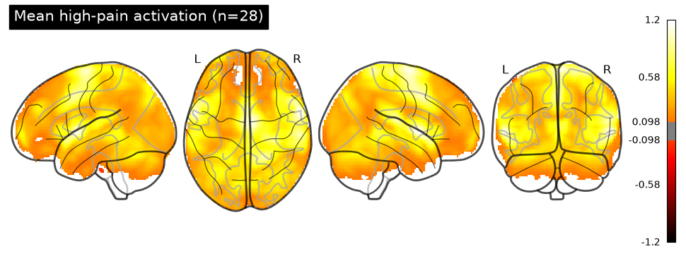

One-sample group t-test¶

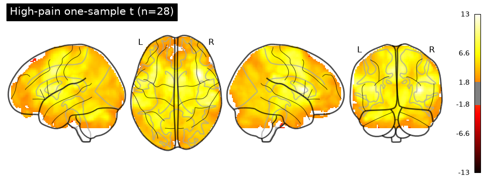
With one map per subject (our high_pain collection), ttest() runs a voxel-wise one-sample t-test across subjects — the classic second-level analysis. It returns a dict of BrainData maps (mean, t, z, p), mirroring BrainData.ttest().

group = high_pain.ttest()
print("returned maps:", list(group.keys()))
group["t"].plot(title="High-pain one-sample t (n=28)")

returned maps: ['mean', 't', 'z', 'p']

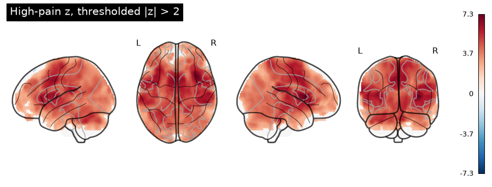
# Threshold the t-map for display (|z| > 2)
group["z"].threshold(lower=-2, upper=2, binarize=False).plot(
    title="High-pain z, thresholded |z| > 2"
)

Where to go next¶

This tour covered the data structure itself — construction, indexing, per-subject parallel ops, the path-backed cache, and group reductions. The full analysis workflows that BrainCollection powers live in the Workflows tutorials:

• GLM Analysis — from_bids → per-subject fit(model="glm") → compute_contrasts(...) → ttest().

• Multivariate Pattern Analysis — cross-subject decoding via bc.predict_group(y, ...) (group MVPA, subjects as samples).

• Inter-Subject Correlation — bc.isc(...) / bc.isc_test(...).

When you’re done with a real (disk-backed) collection, call bc.cleanup() to remove its cache root.